A (car) crash course in embeddings
In the last post, I built a simple neural network for predicting the price of Ford Fiestas using numerical features (mileage, year of registration, and engine size). In this post, I’ll be expanding the predictor to deal with any make and model, and in doing so learning about how to use embeddings to deal with categorical variables.
LLMs and writing
Before jumping in, a note on LLM use. I’ve been using Google Gemini, in conjunction with other reading, to help learn concepts and quickly get code working. Any code I share is going to be a mix of my own work, code written by Gemini or other LLMs, and snippets and concepts taken from other blogs and websites. My priority is learning the big picture and I’m very happy to be able to use LLMs to help with the nitty gritty of the implementation.
On the other hand, all the wording in the blog is entirely my own (nothing is ‘quietly’ doing anything, which seems to be the GenAI word of the week). I find that being deliberate about writing helps my thoughts become more coherent. I also remember things better. In other words, I am aiming to ‘think in ink’, so to speak. Secondarily, I want to avoid ‘semantic ablation’, the phenomenon whereby an author’s unique voice and quirks get smoothed down into an overly polished, generic uniformity. I’m not opposed to using LLMs to help with writing, but to use them for this particular blog would be to miss the point.
I’ve also realised that I tend to use first person plural a lot when writing, e.g. “we train the model on XYZ data”. This is super common in mathematics papers, even when there is only one author, which is no doubt where I picked up this habit. One way this has been explained to me is that I’m bringing the reader along with me, and the “we” is me and them. Anyway, I think it sounds quite natural.
Embedding
So, back to the business at hand. As mentioned in the previous post, the price of a car is definitely going to depend on the make and model, categorical variables which don’t have any obviously meaningful encoding as numbers. A classic way to deal with categorical data is via one-hot encoding. This involves a new column for every possible make of car, with a Ford having a 1 in the Ford column and a 0 in the Volvo column and everywhere else. If we have around 100 makes, each with even 50 possible models, we’ve gone from 2 variables to 5000, and we’re keeping track of huge arrays of mostly zeroes. Even I can see this is not an efficient use of memory. Furthermore, this wouldn’t allow us to capture the fact (or expectation at least) that a Ford Fiesta should be close in price to a Vauxhall Corsa (say) and far from some small BMW hatchback*, even if the mileage and age were the same.
*You may have noticed by now that I don’t know much about cars…
A cool way to approach this kind of categorical data with many options is via embeddings. Using the example at hand, each car make is represented as an element of a real Euclidean space of a sensible dimension (say 5 or 10). So we represent the makes as dense vectors of floating point numbers in low dimensions instead of sparse vectors of 1s and 0s in high dimensions. Straightforward enough. This deals with the dimensionality problem. Of course, now our feature is encoded numerically! So our neural network can do its usual thing and try to learn how price depends on where the values of ‘make’ are mapped in the vector space. By calculating the loss function and using backpropagation in the usual way, the model adjusts the embedding of each car make until it arrives at a configuration where similarly priced models are close together in space.
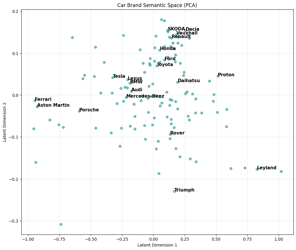
We can actually have a look at this configuration. In my new and improved price predictor, the models are mapped to a 10 dimensional space. Visualising 10 spatial dimensions is hard (at least for me), but we can do some Principle Component Analysis (thanks Gemini) and plot the so-called ‘semantic space’ of car models in 2 dimensions. Its hard to say what the dimensions really mean, but we do see that brands occupying a similar market niche are close to each other.
When training the Fiesta-only model, we used engine volume as a feature. However, the full training data includes EVs where engine volume doesn’t make sense. So the new version uses make, model, variant (a.k.a. trim, e.g. ‘GT’, ‘Titanium’) and fuel type as categorical features (along with mileage and year of registration as numerical features). The categorical features are each embedded into their own vector space, and then their concatenation, just a longer vector, is fed into the model.
A pedantic mathematical detour
Readers with a maths background like me might be wondering if the theoretical map from the high-dimensional space to the low-dimensional space is truly an embedding, in the sense of being injective (a.k.a. one-to-one). That is, is it guaranteed that Ford and Ferrari don’t map to the same point?
Or crash! The proper terminology is in fact a collision.
The allocation of the initial vector for each possible value is actually random, so there is technically a chance that the cars collide. But picking something like 100 floating point vectors in 10 dimensions, even if constrained to be small, is incredibly unlikely to result in collisions, so we can be pretty confident that the Embedding is really an embedding in the mathematical sense.
Implementation
The updated model also has some other bells and whistles.
- The model is trained to predict the log of the target values. This means its minimising percentage error rather than absolute error, which helps with the small number of very expensive cars in the dataset.
- An adaptive learning rate helps converge on accurate predictions more efficiently. We start with a higher rate, taking larger steps. Once we hit a plateau in the loss function, we reduce the rate and take smaller steps to try to dig deeper.
- If the loss function fails to decrease for a long enough stretch, the training will terminate so that it doesn’t continue running through more epochs without making improvements.
- We use ‘dropout’, a standard technique to reduce overfitting. I should write about this in a future blog post.
Here is a very loose sketch of how the implementation goes.
The training data is from the same Kaggle dataset as the last post: UK Used Car Listing Data.
Once the data is cleaned and the random slices for validation (during training) and testing (after training) have been reserved, we set up vocabularies for each categorical feature. These are just dictionaries assigning an integer to each value (Mercedes-Benz maps to 1, Ford maps to 2 etc).
The 4 categorical inputs are encoded as arrays of integers according to the vocabularies. These are then combined into a dictionary with the 2 arrays of numerical inputs (mileage and registration year). This dictionary will be passed to the model as training data (if we name the input layers in the model with the same names as the dictionary keys, the Keras’ fit() function knows to match them up correctly).
In the model, we have the following layers:
- 4 1-dimensional
Inputlayers for make, model, variant, fuel type. - 4
Embeddinglayers of appropriate dimensions which map the vocabularies to small random vectors. - 1 2-dimensional
Inputlayer for the numerical inputs. - 1
Normalizationlayer, adapted to the numerical inputs, to unify the mean and variance. - 1
Concatenatelayer to merge the 5 feature layers - 2
Denselayers, with ReLu activation functions, for the actual neural network magic. - 2
Dropoutlayers, one after each Dense layer, to help reduce overfitting. - 1
Denseoutput layer, with linear activation.
We train the model using Mean Square Error, which is the standard approach for log space targets.
You can see the code on github.
Results
Testing the trained model on the reserved set of test data, we get the following graphs.
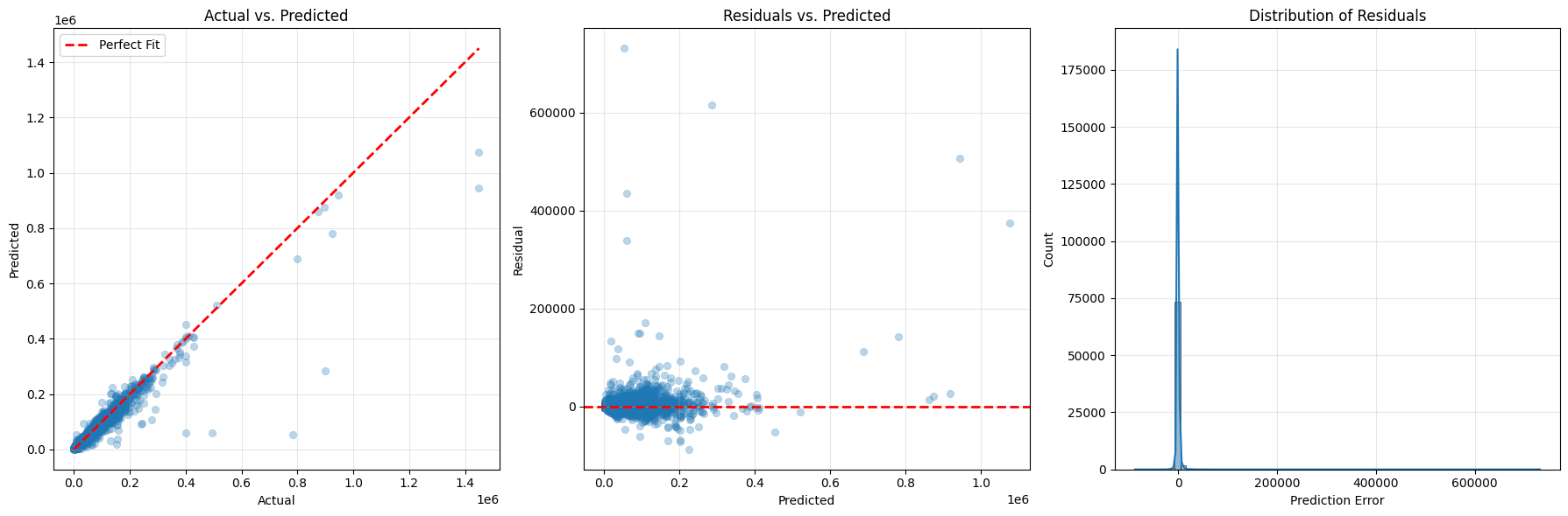
For the most part, I think we’ve got a pretty good predictor here. The distribution of errors is very tall and thin, meaning the vast majority of errors are small. We just have a small number of really very outlying outliers.
Conclusion
The embedding layer provides a slick way of encoding many-valued categorical data into a neural network in a way that is computationally efficient, and enables the network to learn the relative position of different values within a ‘semantic space’, lending more precision to future predictions.
As I mentioned in my previous post, I am expecting a regional factor in car prices. This is definitely something I will explore in future, and try to factor this in to the model training.
For now, though, I think my next step will be to put together a web interface and link it up to this price predictor that I’ve trained, trying to imagine what a real-world user might want.