How much is this Ford Fiesta worth?
Suppose that I’m looking for a car to buy. I’ve found one advertised by a local dealership or a private seller. How can I gauge if the price is fair? What I would like is a tool where I can input the car details and find out how fair the price looks, in terms of the current market conditions. My plan is to build such a tool, as a (hopefully) fun learning exercise. And blog about it along the way to document my process and to keep myself accountable.
I’m going to start from the middle and build out in all directions. First up is the machine learning. The plan is to build a price predictor using Python (Pandas, TensorFlow, Keras), which can be trained on recent market data. Then for a new advert that comes along, a prospective buyer can compare the listed price against the predictor and decide whether it’s above or below the expected price. Alternatively, a seller could use this kind of model to determine how to price their car.
Data
I need some training data. The first source that came to mind was Autotrader. However, it turns out that its not so easy to get access via their API and apparently they aren’t keen on scrapers. For now, Kaggle user Guanhao Peng has the answer in the form of their dataset UK Used Car Listing Data (which looks suspiciously like it came from Autotrader…).
I’m starting very small and just looking at Ford Fiestas. They’re a very popular choice in the secondhand market in the UK (indeed, I own one) so there is plenty of data. I’m hypothesising that mileage, year of registration, and engine volume might be enough info to determine a decent price prediction. There is more to the various kinds of Fiestas than just engine volume, but that is categorical and for this initial step I just want to focus on numerical data.
Cleaning
Once I had the data in a pandas DataFrame, there was a wee bit of cleaning to do. There were some rows with missing year and registration data. I couldn’t see a way of filling in the missing info, so these rows were discarded. After that, there were somewhat more than 12000 Ford Fiestas left in the dataset. Of these, 20 had missing engine volumes, few enough to look at individually. There were 14 cases where the engine volume was in a free text description field, so they could be added. The other 6 were discarded. There were also some rows with missing mileage. Again, these were discarded.
Initial Analysis
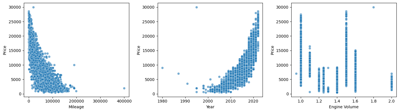
After splitting off 20% of the rows to use for testing the model, I explored the relationships between price and my chosen features. As can be seen in the following scatterplots, there are clearly (non-linear) relationships between mileage and price, and between year and price. Engine volume is a bit less clear, but it doesn’t seem to be random. It did make me think about whether this feature should really be categorical. Something to play with in the future. For now, we’ll keep it numerical, just in case we need to predict the price of a Fiesta whose engine volume is \(\sqrt{2}\) litres!
Training the model
I experimented with simple neural networks with different numbers of hidden layers. I used ReLU for the activation functions of the hidden layers (since its straightforward and computationally efficient), and also for the output layer (since I want a non-negative price at the end of the day). I’m probably training for more epochs than necessary (400), but I want to be sure that the model has wrung as much learning as possible from the data. I played around with different learning rates and settles on a uniform 0.05 across the different versions.
Here are some charts describing the results of training models with 0, 1, 3, 5 hidden layers respectively. On the left we have the changing loss function throughout the model’s training, with the orange line marking validation against 20% of the data. We then look at how the model fared when predicting the prices of the cars it was not trained on. First, we plot predicted price against actual price, then residuals (i.e. the difference between the prediction and the true price) against actual price, and finally the distribution of residuals. We also output the overall mean squared error (MSE). I’m not sure how useful this single figure is, but it does give a way of comparing the models’ performance.
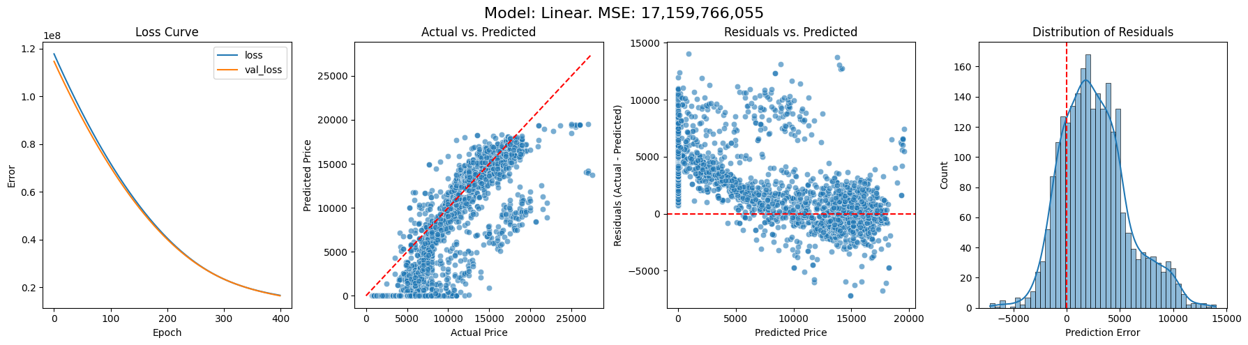
Without hidden layers, we are essentially trying to fit a single linear (well, almost) function, which does not go well (unsurprisingly given the scatterplots above). This model under-prices lots of cars by a significant amount.
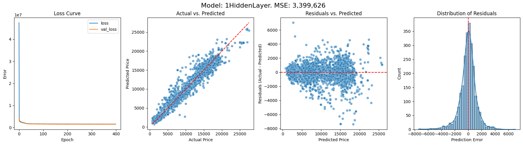
With just 1 hidden layer we are already getting something much more convincing. The fact that there isn’t a pronounced fan shape on the Residuals vs Predicted chart suggests that there is not much loss of accuracy as the price increases. The Distribution of Residuals is pretty tall and thin, meaning they’re mostly small, and its pretty symmetric about zero, so the model isn’t biased towards under- or over-pricing.
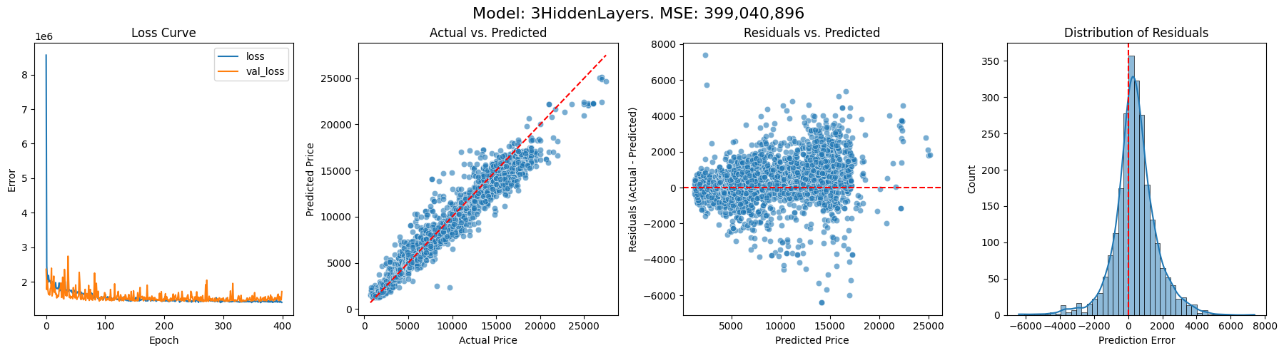
With 3 hidden layers, the general shape is unchanged, but we seem to have a bit of a bias for under-pricing.
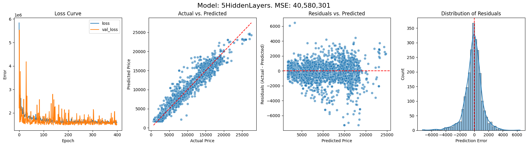
With 5 hidden layers, the bias has disappeared. However, it doesn’t seem to be significantly better at predicting the price than just a single hidden layer, and the MSE is much larger. Interestingly, in a previous run of the same models, the model with 3 hidden layers was the best performer. It seems likely that the specifics of the number of layers is probably not significant here, and just having a decent number of nodes pretty much finds everything that can be found from these 3 training features. For more accuracy, we probably want to incorporate other features.
Code
If you’re interested, the github repo is here, with a nice clean version of the code entitled “blog_1102.ipynb”.
Next steps
From personal experience, I know that the location of the car can also impact the price. The last time I bought a car, I was working in Manchester, and I found significantly better prices there than I could find at home in Edinburgh. So for one of the next steps in this project I’d like to take this into account. The data includes the location as a string so perhaps I can map that to coordinates and incorporate that into the training.
I also need to deal with every make/model of car. We could train a seperate neural network for each type of car, but there are too many for that to be practical. Clearly, a Ford and a BMW of the same age with matching mileages and engine sizes are not going to cost the same. So we should include this categorical data as a feature. Since there are so many possible make/model combinations, one-hot encoding is going to give a high-dimensional input layer, and also not capture any similarities between similar models of car. So an embedding layer might be the way to go. This is a way of teaching the neural network to represent makes/models as points in a smallish-dimensional continuous vector space. As well as keeping the dimension manageable, this also gives the model a chance to learn that, say, a Ford Fiesta is “close to” a Vauxhall Corsa, but “far away from” a Porsche Cayenne. More on this in a future blog post!
If you have any advice for getting up-to-date data on car prices from the real world, I’d love to hear it! You can reach me via LinkedIn.